MS Excel आज लगभग हर Office, School, Business और Company में उपयोग किया जाता है। Excel में कई ऐसे Powerful Features होते हैं जो Data को समझना और Analyze करना आसान बनाते हैं। उन्हीं में से एक महत्वपूर्ण Feature है Conditional Formatting।
Conditional Formatting की मदद से आप Data को Automatically Highlight कर सकते हैं। इससे Important Values, Duplicate Entries, Low Marks, High Sales या Pending Records तुरंत पहचान में आ जाते हैं।
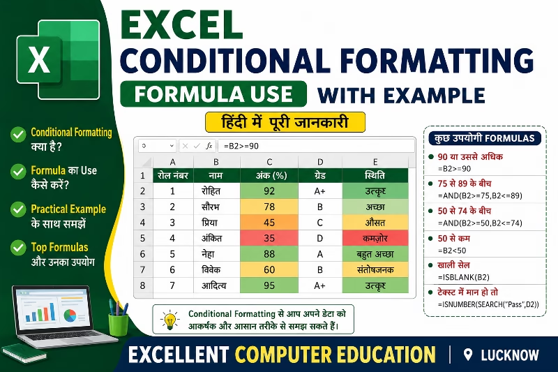
लेकिन जब आप Conditional Formatting में Formula का उपयोग करना सीख जाते हैं, तब Excel और भी ज्यादा Powerful बन जाता है। इस लेख में हम Conditional Formatting Formula को आसान भाषा में Example के साथ समझेंगे।
Conditional Formatting क्या है?
Conditional Formatting Excel का ऐसा Feature है जो किसी Condition के अनुसार Cells का Color, Font या Style Automatically बदल देता है।
उदाहरण:
90 से अधिक Marks को Green Color
कम Sales को Red Color
Duplicate Data को Highlight करना
Conditional Formatting Formula क्यों उपयोग करें?
Normal Conditional Formatting केवल Basic Rules तक सीमित होती है। लेकिन Formula की मदद से आप:
- Custom Conditions बना सकते हैं
- Multiple Criteria Use कर सकते हैं
- Dynamic Highlighting कर सकते हैं
- Professional Reports तैयार कर सकते हैं
Conditional Formatting Formula लगाने का तरीका
Step-by-Step Process
- Data Select करें
- Home Tab में जाएं
- Conditional Formatting पर Click करें
- New Rule चुनें
- “Use a Formula to Determine Which Cells to Format” चुनें
- Formula Enter करें
- Format Select करें
- OK पर Click करें
Example 1: 5000 से अधिक Sales Highlight करें
मान लीजिए आपके पास Sales Data है:
| Product | Sales |
| Laptop | 4500 |
| Printer | 7000 |
| Mouse | 3000 |
| Keyboard | 6500 |
अब हमें 5000 से ज्यादा Sales को Highlight करना है।
Formula:
=B2>5000
Result:
7000 और 6500 वाले Cells Highlight हो जाएंगे।
Example 2: Duplicate Values Highlight करें
अगर Data में Duplicate Entries हैं, तो उन्हें Highlight करना बहुत जरूरी होता है।
मान लीजिए Employee IDs की List है।
Formula:
=COUNTIF(A:A,A1)>1
Result:
जो भी ID एक से ज्यादा बार होगी, वह Highlight हो जाएगी।
Example 3: पूरे Row को Highlight करें
मान लीजिए Attendance Sheet में “Absent” Students की पूरी Row Highlight करनी है।
| Name | Status |
| Rahul | Present |
| Amit | Absent |
| Neha | Present |
Formula:
=$B2=”Absent”
Result:
जिस Row में “Absent” होगा, पूरी Row Highlight हो जाएगी।
Example 4: आज की Date Highlight करें
अगर किसी Sheet में आज की Date Highlight करनी हो:
Formula:
=A1=TODAY()
Result:
आज की Date वाला Cell Automatically Highlight हो जाएगा।
Example 5: Odd और Even Numbers अलग दिखाएं
Even Number Formula:
=MOD(A1,2)=0
Odd Number Formula:
=MOD(A1,2)=1
Result:
Even और Odd Numbers अलग-अलग Color में दिखेंगे।
Conditional Formatting Formula उपयोग करते समय जरूरी बातें
Cell Reference सही रखें
- गलत Reference देने से Rule सही काम नहीं करेगा।
Dollar Sign ($) का सही उपयोग करें
- $A$1 = Fixed Cell
- A1 = Relative Cell
यह Formula Behavior को नियंत्रित करता है।
Data साफ रखें
- Blank Rows और गलत Data होने पर Formatting सही नहीं दिख सकती।
Conditional Formatting के फायदे
- Important Data जल्दी पहचानना
- Errors कम करना
- Reports को Professional बनाना
- Time बचाना
- Data Analysis आसान करना
Conditional Formatting कहाँ उपयोग किया जाता है?
Conditional Formatting का उपयोग:
- School Reports
- Attendance Sheets
- Sales Reports
- Accounting
- Inventory Management
- HR Reports
- Dashboard Creation में किया जाता है।
निष्कर्ष
Conditional Formatting Formula Excel का एक बहुत Powerful Feature है जो आपके Data को Smart और Professional बनाता है। इसकी मदद से आप बड़े Data को आसानी से Analyze कर सकते हैं और Important Information तुरंत पहचान सकते हैं।
अगर आप Excel में Expert बनना चाहते हैं, तो Conditional Formatting Formula सीखना आपके लिए बहुत जरूरी Skill हो सकती है। Regular Practice और सही Examples की मदद से आप इसे आसानी से सीख सकते हैं।